F-distribution
| Probability density function |
|
| Cumulative distribution function |
|
| Parameters |  deg. of freedom deg. of freedom |
|---|---|
| Support |  |
 |
|
| CDF |  |
| Mean |  for for  |
| Mode | 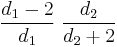 for for  |
| Variance | 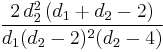 for for  |
| Skewness | 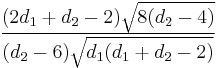 for  |
| Ex. kurtosis | see text |
| MGF | does not exist, raw moments defined in text and in [1][2] |
| CF | see text |
In probability theory and statistics, the F-distribution is a continuous probability distribution.[1][2][3][4] It is also known as Snedecor's F distribution or the Fisher-Snedecor distribution (after R.A. Fisher and George W. Snedecor). The F-distribution arises frequently as the null distribution of a test statistic, most notably in the analysis of variance; see F-test.
Contents |
Definition
If a random variable  has an F-distribution with parameters
  and
and  , we write
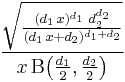
  . Then the probability density function for is given by
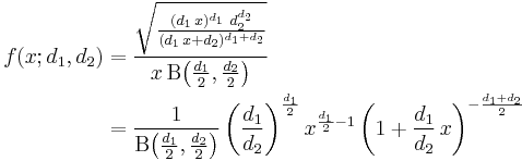
for real  . Here
  is the beta function. In many applications, the parameters and are positive integers, but the distribution is well-defined for positive real values of these parameters.
The cumulative distribution function is
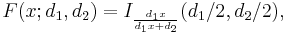
where I is the regularized incomplete beta function.
The expectation, variance, and other details about the  are given in the sidebox; for
  , the excess kurtosis is
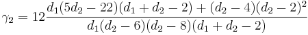 .
.
The k-th moment of an distribution exists and is finite only when  and it is equal to [5]:
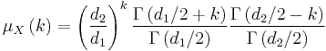
The F-distribution is a particular parametrization of the beta prime distribution, which is also called the beta distribution of the second kind.
The characteristic function is listed incorrectly in many standard references (e.g., [2]). The correct expression [6] is
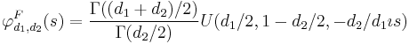
where  is the confluent hypergeometric function of the second kind.
Characterization
A random variate of the F-distribution with parameters d1 and d2 arises as the ratio of two appropriately scaled chi-squared variates:

where
- U1 and U2 have chi-squared distributions with d1 and d2 degrees of freedom respectively, and
- U1 and U2 are independent.
In instances where the F-distribution is used, for instance in the analysis of variance, independence of U1 and U2 might be demonstrated by applying Cochran's theorem.
Generalization
A generalization of the (central) F-distribution is the noncentral F-distribution.
Related distributions and properties
- If
 and
and  , and are independent, then
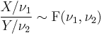
- If
 (Beta-distribution) then
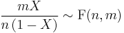
- If
 then
then  has the chi-squared distribution
 is equivalent to the scaled Hotelling's T-squared distribution
  .
.- If
 then
then  .
. - If
 (Student's t-distribution) then
  .
. - If
 (Student's t-distribution) then
  .
. - F-distribution is a special case of type 6 Pearson distribution
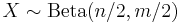
- If
 and
and  then
then  has a Beta-distribution.
- If X and Y are independent, with
 and
and  (Laplace distribution) then
- If
 then
then  (Fisher's z-distribution)
 - The noncentral F-distribution simplifies to the F-distribution if

- The doubly noncentral F-distribution simplifies to the F-distribution if
- If
 is the quantile
  for and
  is the quantile
  for
for  , then
-
 .
.
References
- ^ a b Johnson, Norman Lloyd; Samuel Kotz, N. Balakrishnan (1995). Continuous Univariate Distributions, Volume 2 (Second Edition, Section 27). Wiley. ISBN 0-471-58494-0.
- ^ a b c Abramowitz, Milton; Stegun, Irene A., eds. (1965), "Chapter 26", Handbook of Mathematical Functions with Formulas, Graphs, and Mathematical Tables, New York: Dover, pp. 946, ISBN 978-0486612720, MR0167642, http://www.math.sfu.ca/~cbm/aands/page_946.htm.
- ^ NIST (2006). Engineering Statistics Handbook - F Distribution
- ^ Mood, Alexander; Franklin A. Graybill, Duane C. Boes (1974). Introduction to the Theory of Statistics (Third Edition, p. 246-249). McGraw-Hill. ISBN 0-07-042864-6.
- ^ Taboga, Marco. "The F distribution". http://www.statlect.com/F_distribution.htm.
- ^ Phillips, P. C. B. (1982) "The true characteristic function of the F distribution," Biometrika, 69: 261-264 JSTOR 2335882
External links
- Table of critical values of the F-distribution
- Earliest Uses of Some of the Words of Mathematics: entry on F-distribution contains a brief history
|
|||||||||||